Changing the format of results

After you create a query in Explore, you can change the format of your results to percentages, currency, timestamps, or custom formats using the Display format option in the chart configuration () menu. This article shows you how to set your results to one of Explore's pre-built formats or create your own customized format.

This article contains the following sections:

• Changing results to a pre-built format
• Customizing the result format
• Adding conditional formatting for tables

Changing results to a pre-built format

Explore automatically offers pre-built formats for your results. This section will describe each pre-built format and how to access them.

To change your result format

1. In query builder, click the chart configuration icon ().
2. Select the Display format option.
3. Click the drop-down list next to your metric. By default, all results are in standard format.
4. Select a format option. There are five pre-built options:

   

   • $: Reformats your results into dollars. If your results contain decimal numbers, they will be added as cents.
   • €: Reformats your results into euros.
   • %: Multiplies your results by 100 and adds the percentage symbol (%).
     Note: If you do not want to multiply your results by 100, you can add a percentage suffix as a custom format (see Customizing your result format).
   • Finance: Displays two decimal values. If your results do not include any, two zeros will be added after the decimal point.
   • Duration: Convert your results into the dd:hh:mm timestamp (days, hours, minutes). Your metric can only be converted into dd:hh:mm.

   Your results are automatically converted to the selected format.

Customizing the result format

Use this section to learn about custom formatting options. You can use the steps in the section above to change your result format to the Custom option. If you want to display separate formatting, for different ranges of value in the same metric, you can use the Advanced option. See Adding conditional formatting.

To customize the result format

1. In Query Builder, click chart configuration ().
2. Select the Display format option.
3. Click the drop-down list next to your metric. By default, all results are in standard format.
4. Select Custom.

You can customize your results with the following formatting options:

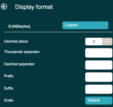
• Decimal place: Add or remove decimal places from your results. If your results do not contain decimal numbers, zeros will be added to your results.
• Thousands separator and Decimal separator: Enter a symbol to represent every thousand or the decimal point.
• Prefix and Suffix: You can add a symbol to the beginning or end of your result without altering your numbers. The suffix option is useful if you want to display your results as a percentage, but do not want to multiply by 100.
• Scale: Divides your results by your selected option. You can select the following:
  • 0.01 and 0.01
  • Thousands, Millions, Billions, and SI Units

Adding conditional formatting for tables

For tables, you can display different formatting based on specified set of conditions, by selecting the Advanced option. With the Advanced formatting option, you can create new and edit existing IF THEN ELSE statements with your metric conditions and resulting formatting.

To apply conditional formatting for tables

1. In Query Builder, click chart configuration ().
2. Select the Display format option.
3. Click the drop-down list next to your metric. By default, all results are in standard format.
4. Select Advanced.

The following are the formatting options you can apply:

• backgroundColor: Set the background color. Colors are represented by six digit HEX code.
• precision: Add or remove decimal places to your results. If your results do not contain decimal numbers, zeros will be added.
• scale: Divide your results by your selected option. For example, you can view your results to the thousandths by dividing by a thousand.
• prefix: Enter a symbol to appear in the front of values.
• decimalSeparator: Enter a symbol to represent the decimal point.
• italic: Enter TRUE to present values in italics, or FALSE to present them in regular font.
• bold: Enter TRUE to present values in bold, or FALSE to present them in regular text.
• suffix: Enter a symbol to appear at the end of values.
• fontColor: Set the text color. Colors are represented by six digit HEX code.
• thousandsSeparator: Enter a symbol to represent every thousand.

Note: If you do not add one of the formatting options to your THEN statement, that option will render as the default.

The following query example uses conditional formatting to highlight the number of open tickets each agents have and quickly identify agents with an outstanding number of open tickets. Agents

The query uses the following formula to generate these results:

IF (COUNT(# Open Tickets) > 25) THEN
    {
        "backgroundColor": "#FF5733",
        "precision": 0,
        "scale": 1,
        "prefix": "",
        "decimalSeparator": ".",
        "italic": FALSE,
        "bold": TRUE,
        "suffix": "",
        "fontColor": "",
        "thousandsSeparator": " "
    }
ELIF (BETWEEN((COUNT(# Open Tickets)),10,25)) THEN
    {
        "backgroundColor": "#FFC300",
        "bold": TRUE
    }
ELIF (COUNT(# Open Tickets) <10) THEN
    {
        "backgroundColor": "#19C700 ",
        "bold": TRUE
    }
ENDIF

For additional resources for writing formulas in Explore see Formula writing resources